Seismically-induced tidal waves, or tsunamis:
Diagnostic sediments deposited along coastal lowlands; funnel-shaped inlets particularly vulnerable; coral found in canyons up to 400 m above sea level in the Hawaiian Islands. Hilo, Hawaii is the tsunami capital of the world. M8.9 Chilean earthquake in May 1960 left similar evidence as massive Cascadia Subduction Zone quake in early 1700 along the coast of Oregon and Washington. In each instance, the sea floor was subducted about 200 meters! Seismically-induced seich killed thousands in Japan in 1700.
Sinking of RMS Titanic in April 1912.
Unusually warm winter causes increased iceberg calving at Disco Bay, Greenland and brings the cold Labrador current further south into warm north Atlantic Gulf stream than in previous 40 years. Titanic’s Captain Edward J. Smith was the highest paid mariner in the world and the most experienced ship’s captain on the North Atlantic at the time, having commanded ships along those sea lanes for 25 years. He didn’t take iceberg warnings as seriously as he should have and forgot to account for the southward drift of those sightings that were plotted on the navigation bridge.
The environmental conditions surrounding the Titanic’s untimely demise were extremely rare: the night was moonless; the sea temperature was 29 degrees Fahrenheit and the Titanic’s fresh water bilges were freezing up. There were no waves, the ocean was at Sea State 1, unusually calm, “like a millpond”. These windless and waveless conditions prevented phosphorescent wave wash against the icebergs, which was how they were normally identified at night by watchmen stationed in the crow’s nest, about 120 feet above the water. With binoculars the watchmen were usually able to identify icebergs at ranges of between 6,000 and 2,000 yards. The watchmen were without binoculars that evening because they had unknowingly been stowed in the Second Officer’s cabin. The speed of the ship was about 22.5 kts and the wind chill factor on the watchmen would have been about would The iceberg that sank the Titanic was not identified until the ship was within about 500 yards of the ship These unusual metrological conditions were not repeated until 1956, 44 years after Titanic suck.. We now believe that the conditions were probably a 1 in 40 year occurrence
Colorization of Old Photos and Terrestrial Photogrammetry to Solve the 1928 St. Francis Dam Failure
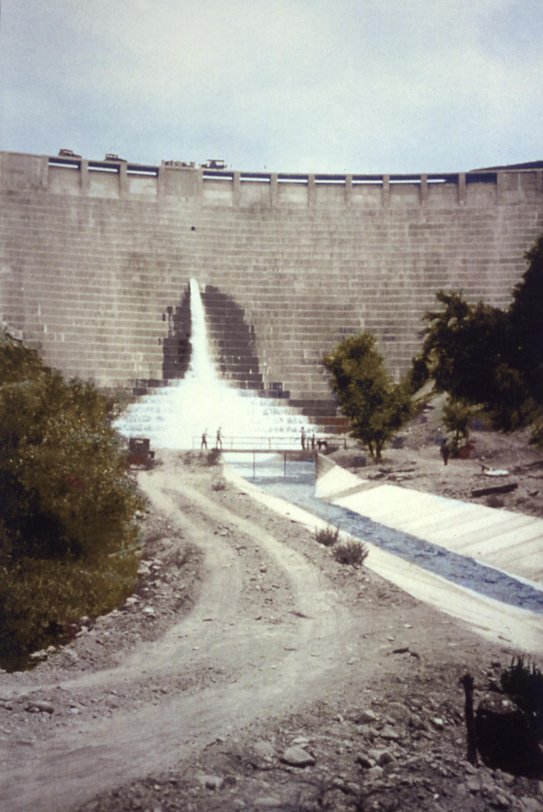
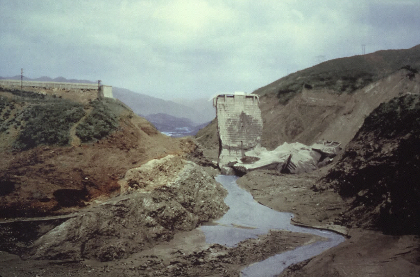
St. Francis Dam was a 200 feet high curved concrete gravity arch dam built by the City of Los Angeles Department of Water and Power in 1924-26 to store a year’s supply of water for the city along their Owens River Aqueduct (completed in 1913). The reservoir was filled to its maximum capacity of 38,180 acre-feet on March 7, 1928, making it the largest reservoir in southern California at the time. Near midnight on March 12/13, 1928the dam suddenly gave way, spilling forth a massive deluge of water, which killed over 435 people as it rampaged seven miles down San Francisquito Canyon, thence into the Santa Clara River to the Pacific Ocean, 52 miles away.
Post-failure assessments were undertaken by no less than a dozen prestigious boards of consultants. Most of these studies were of a cursory nature and did not take into consideration independently-collected data fro the scene of the failure. Most of the investigative boards blamed the failure on the presence of a dormant fault beneath the dam’s right abutment and chastised the dam’s chief engineer for not obtaining expert geologic input before sitting the dam and not having the design reviewed by an independent panel of experts. In the wake of public outcry following the disaster, California amended its dam safety law to include State overview of all dams and reservoirs, except federally owned facilities (which were automatically subject to similar peer review). They also instituted statewide registration of civil engineers.
In the late 1960s I became interested in the St. Francis Dam failure through its portrayal in a news program that profiled southern California history. I visited the dam site with my college field geology class in 1974, and began thinking about re-evaluating the failure after discussing the case with one of my graduate advisors at Berkeley, who was a world renown expert in concrete dams. During graduate school (1976-82) I worked on unraveling the June 1976 failure of the Teton Dam near Rexberg, Idaho. During my post-graduate years I worked in forensic engineering as a Naval intelligence officer. In doing so I was exposed to many specialized techniques of obtaining valuable field data, even from old photographs and maps.
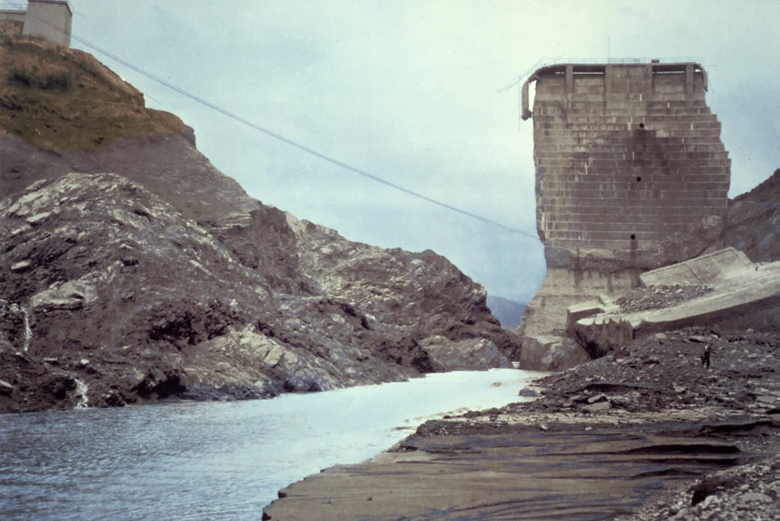
One tried-and-tested technique is to make careful measurements on photos taken after the collapse. These are akin to photos imaged at a crime scene: they hold many valuable clues, but after seventy-five years, much has changed at the site, including the "tombstone" slab, demolished in 1929. Today new growth obscures evidence of the scour lines that the flood left on the canyon walls. In the 1928 photographs they are clearly seen, indicating how high the water was. In order to estimate the size of the flood in 1928, it is necessary to make accurate measurements on the old photos. To do that, I went out to the site with a 35mm camera, a Global Positioning Satellite receiver, and sets of post-collapse photographs. I then employed photographic analysis techniques that date to mid-19th Century Germany, based on an Ancient Greek discovery, parallax, or difference in viewing angles.
The first step is to locate where the 1928 photographer stood and the kind of lens he used. By comparing what I saw through my camera and the existing photographs I was able to can accomplish this. Next, I used a hand-held GPS receiver to locate visible landmarks on both the photograph and the site today. Knowing the distance from that landmark, I e take a picture, the calculate a 1 degree parallax, or viewing angle, and pace off that distance and takes a companion photograph. For example, an object 1000 feet away would require images taken 17.5 feet apart. Now, the two images form a "stereo pair" of photographs, like the popular stereo-opticons of the 19th century. Using stereopairs to the 1928 images, I was then able to calculate the relative position, heights and distances of objects in the old photos. As many as 100 photographs were used in this stage of the analysis. In the end an accurate map of the site before and after the collapse was created.
Making stereopairs for the 1928 photos is a fundamental starting point in any forensic analysis. These allow accurate measurement of identifiable fragments, such as the displaced pieces of the dam. Previous investigators gave each block a number -- from 1 to 44. Knowing where these blocks ended up after the disaster, and where they came from is vital to understanding the sequence of the collapse.
If there was a landslide of the dam’s left abutment, what role did it play? The disintegrating sandstone on the west abutment captivated early investigators. All of the evidence clearly points to the east abutment as the starting point of the disaster. Using a technique employed to "colorize” Hollywood movies, I had several of the 1928 photographs treated in this manner. A Multispectral Scanner was employed to record the precise wavelengths of visible light emitted by various features at the site, such as the rocks, concrete fragments, plants, trees and water. This data allowed a computer simulation of the colors formerly seen as various shades of grey in the old black and white photos. The colorization allowed water and sediment in the reservoir to be distinguished from one another, something previously overlooked. These markers indicate that the collapse clearly started on the east abutment and that the water was surprisingly low before the west abutment failed. As much as 75% of the reservoir's water was gone before the west abutment failed.
Supporting this, perhaps the single most dramatic clue came from the Steven’s Gage, a device that measures the absolute elevation of the reservoir pool, using the water pressure on a submerged pipe, extending some 70 feet below the upstream face of the dam. The gage recorded a curious but progressive drop of the reservoir pool, beginning around 8 o’clock the evening of the midnight failure, then a sharp and abrupt drop near midnight, when the dam went out. If the reservoir actually dropped the 3-1/2 inches or so suggested by the gage, an enormous outpouring of water would have occurred, but none was noted by the survivors and eye-witnesses that drove up the canyon during this same interim. For these reasons, most post-failure investigators refused to believe that the gage’s clock mechanism was accurate, and Stevens Gage became a mysterious footnote to the terrible tragedy.
But, an alternative explanation was apparently overlooked. Instead of the reservoir falling, the dam was actually tilting. Using computerized structural mechanics analyses, I was able to show how the thrust of the slowly slipping mountain, weighing about five times as much as the dam, could have tilted the dam by as much as 1.75 feet, causing the reservoir pool to “drop” the 3.5 inches recorded by the Stevens Gage! A tilt of 1.75 feet over the dam’s face height of 200 feet only requires a tilt of 0.50 degrees!
This work was initially published in 1992 and was well received by the engineering community, for which I was accorded the E.B. Burwell Award of the Geological Society of America and the 1994 Rock Mechanics Award of the National Research Council. In 1995 I published a more extensive explanation of the disaster and some of the methods used to unravel the failure, suggesting the term “geoforensics” be applied to that portion of forensic engineering that deals with earth and ocean systems. This later work was recognized with the 1996 R.H. Jahns Distinguished Lectureship Award of the Association of Engineering Geologists and geological Society of America and the 1999-2001 appointment to the Society of Sigma Xi College of Distinguished Lecturers. In July 2001 I left the Department of Civil & Environmental Engineering at the University of California, Berkeley to accept the Karl F. Hasselmann Chair in Geological Engineering at the University of Missouri-Rolla.
Colorized Images of
The St. Francis Dam Before And After Failure.
Questions or comments on this page?
E-mail Dr. J David Rogers at rogersda@mst.edu.
![]()