Aquifer Detection
and Characterization by Material Balance Methods in the Niger Delta
The objective of this project is to detect the presence of as well as characterize the relative strengths of aquifers associated with oil fields in the Niger Delta using Material Balance methods.
It has long been known that the concept of Material Balance Equation (MBE) as a straight line can be used to determine the Initial hydrocarbon in place (IHIP) as well as detect the presence of aquifers associated with oil and gas reservoirs. Recently however, Pletcher(1) has shown that the conventional MBE methods can be adapted to characterize the relative strengths of these aquifers (whether weak, moderate or strong). In this work, the validity of these adaptations will be tested by application to Niger delta oil fields. Specifically, the Campbell plot will be used to identify the relative strengths of Niger Delta aquifers. Where applicable, the Pot-aquifer plot will be used to determine aquifer water volume where formation compressibility is known.
Campbell Plot
The generalized material balance equation for oil reservoirs can be expressed in the form(2 ):
This equation can be put in a more compact form by making the following designations:
Let;
Introducing these terms into the MBE equation allows it to be written as:
![]()
Furthermore, if we let ![]()
Then the MBE equation can be further simplified to be of the form:
![]()
Note that one could also have arrived at identical results if one had used the following definitions:
Reservoirs under volumetric depletion
For volumetric reservoirs, ![]() = 0 and therefore
= 0 and therefore ![]() indicating that the
original oil in place (N) can be calculated directly as:
indicating that the
original oil in place (N) can be calculated directly as: ![]() . Thus, the value of N can be calculated at every pressure
where production data is given. If this is done, the theory says that if the
reservoir is truly under volumetric depletion, then the calculated values of
. Thus, the value of N can be calculated at every pressure
where production data is given. If this is done, the theory says that if the
reservoir is truly under volumetric depletion, then the calculated values of ![]() should give the same
constant value at all pressures. In practice, this is often not the case either
because there is water influx or because there may be faulty pressure or
production readings.
should give the same
constant value at all pressures. In practice, this is often not the case either
because there is water influx or because there may be faulty pressure or
production readings.
Analysis procedure
for initially under-saturated reservoirs
Step1: Make a Campbell plot
Since whether or not water influx exists will not be known ahead
of time, the first step is to assume that there is no water influx (i.e. the
reservoir is undergoing volumetric depletion). Then calculate the Initial Oil
in Place (N) at every pressure from the equation: ![]()
If the no water influx assumption is correct and assuming
there are no faulty readings, a plot of ![]() versus Np (called the Campbell plot) should give a
horizontal line. In practice however, there will be scatter in the plot but the
best-fit straight line through the data points should be horizontal and its
intercept on the Y-axis should give the correct value of N as illustrated
below.
versus Np (called the Campbell plot) should give a
horizontal line. In practice however, there will be scatter in the plot but the
best-fit straight line through the data points should be horizontal and its
intercept on the Y-axis should give the correct value of N as illustrated
below.
If however, there is water influx, the Campbell plot (F/Et versus Np) would give any one of three possible curves depending on the strength of the aquifer as shown below.
Thus, the Campbell plot can be used to diagnose the existence of water influx. Furthermore, the shape of the plot gives an indication of the relative strength of the aquifer. Even though this plot can also give the value of the original oil in place, it is not very accurate and so is not the recommended for calculating N. Once the aquifer size is diagnosed, other methods exist for finding the original oil in place. These methods are described below.
Step 2: Volumetric reservoir case
For a volumetric reservoir, plot F versus Et. This plot should give a straight line going through the origin the slope of which = N.
Weak water drive case
A weak water drive implies a small aquifer. Assuming aquifer permeability is high with good communication with the reservoir, such aquifers can be represented with the pot aquifer model where it is assumed that any reservoir pressure drop is instantaneously transmitted into the aquifer. Thus, aquifer pressure drop = reservoir pressure drop. This implies steady state water influx where the amount of influx equals the expansion of the water in the aquifer in response the reservoir pressure drop. That is,
![]()
Where W is the aquifer water volume = aquifer pore volume since the water saturation in the aquifer =1.0.
For the weak water drive cases,
a plot of ![]() should give a
straight line with a Y-intercept = N.
should give a
straight line with a Y-intercept = N.
This is the so-called Pot-aquifer plot and it can be used to determine N and the aquifer water volume W.
![]()
The aquifer water volume can be calculated from the slope as:
Moderate and Strong water influx cases
For such systems, unsteady state water influx prevails. For information on how to analyze these cases, refer to my lecture notes on “Applied Reservoir Engineering” chapter 4, section 4.2 on “Material balance as a straight line”. These methods all involve trial and error calculations of water influx. These calculations are extremely tedious without the use of a computer. Therefore, you may ignore this section for now.
Analysis procedure for initially saturated (Gas-cap) reservoirs
See section 4.3.2 in my lecture notes.
Work to be done for project
- Collect data on oil and gas production with time for various Niger Delta reservoirs together with their corresponding PVT reports. An example would look like the table below: Thes data may be obtainable from Shell or any other oil company.
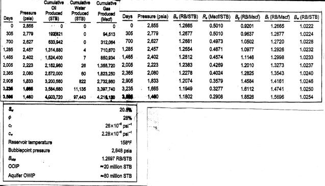
- Make a Campbell plot of the data set for each reservoir and use it to diagnose the relative strength of the associated aquifer.
- If a weak aquifer is diagnosed, make a Pot-aquifer plot and use it to determine the initial oil in place N, and the water volume in the aquifer W.
- By the time you do this for several reservoirs, you would have characterized many of the aquifers associated with Niger Delta oil fields.
- I recommend that you use the data above to practice the procedure described above in steps 1-4.
References
- Pletcher, J. L., “Improvements to Reservoir Material Balance Methods,” SPE Reservoir Evaluation and Engineering (February 2002), 49-59.
- Numbere, D. T., Applied Petroleum Reservoir Engineering, Lecture notes on Reservoir Engineering, University of Missouri-Rolla, 1998.