What
Causes Capillary Pressure?
3.1 EXPRESSIONS
FOR CAPILLARY PRESSURE UNDER STATIC
CONDITIONS
3.1.1 Pc
In terms of radius of capillary tube
3.1.2 Pc
In terms of height of fluid column.
3.1.3 Pc
In terms of radii of curvature of interface
3.1.4 Application
to Parallel Plates
3.2 APPLICATIONS
OF CAPILLARY PRESSURE EXPRESSIONS IN
POROUS MEDIA
3.2.1 Application
to obtain static fluid distribution in porous media
3.2.2 Porous
media modelled as a bundle of capillaries
3.2.3 Porous
media modelled as a packaging of uniform spheres
3.3 Laboratory
methods of measuring capillary pressure
3.3.2 Mercury
Injection Method
3.4.3 Explanations
for capillary hysteresis
3.4.4 The
effect of pore size distribution on capillary pressure curve
3.4.5 Conversion
of Laboratory Capillary Data to Reservoir Capillary Data
3.4.6 Calculating
Average water saturation
3.5 Averaging
Capillary Pressure Curves
3.5.2 How to
use the Leverett J-function to calculate Average Water Saturation
3.5.2.1 Case 1:
Permeability, Porosity, and Elevation are known for each sample
3.5.2.3 Errors due to
using average values of ![]() and
and ![]()
3 CAPILLARY PRESSURE
Reservoir
rock typically contains the immiscible phases: oil, water, and gas. The forces
that hold these fluids in equilibrium with each other and with the rock are
expressions of capillary forces. During waterflooding, these forces may act
together with frictional forces to resist the flow of oil. It is therefore
advantageous to gain an understanding of the nature of these capillary forces.
Definition : Capillary
pressure is the pressure difference existing across the interface separating
two immiscible fluids.
If
the wettability of the system is known, then the capillary pressure will always
be positive if it is defined as the difference between the pressures in the
non-wetting and wetting phases. That is:
![]()
Thus
for an oil-water system (water wet)
![]()
For
a gas-oil system (oil-wet)
![]()
What Causes Capillary Pressure?
Capillary
pressure is as a result of the interfacial tension existing at the interface
separating two immiscible fluids. The interfacial tension itself is caused by
the imbalance in the molecular forces of attraction experienced by the
molecules at the surface as shown below.
For
molecules in the interior:
Net
forces = 0 since there are enough molecules around to balance out.
For
molecules on the surface:
Net
result of forces is a pull toward the interior causing a tangential tension on the
surface.
The
net effect of the interfacial tension is to try to minimize the interfacial
area in a manner analogous to the tension in a stretched membrane. To balance
these forces and to keep the interface in equilibrium, the pressure inside the
interface needs to be higher than that on the outside.
Forces
reducing interface are due to: a)
Interfacial tension
b)
External pressure
The
effect of interfacial tension is to compress the non-wetting phase relative to
the wetting phase. The force created by the internal pressure is balancing it.
3.1 EXPRESSIONS FOR CAPILLARY PRESSURE UNDER STATIC CONDITIONS
3.1.1 Pc In terms of radius of capillary tube
Since
the interface is in equilibrium, force can be balanced on any segment. The
interfacial forces are eliminated by taking as a free body, that part of the
interface not in direct contact with the solid. A force balance would give:
(Internal
pressure - External pressure) * Cross-sectional area = Interfacial tension * Circumference
Thus, ![]()
Therefore, ![]()
And
since by definition, ![]() , we have:
, we have: ![]()
For
an air-water system, the air is the non-wetting phase and ![]()
This
equation is referred to as
3.1.2 Pc In terms of height of fluid column.

![]() because there is no
capillary pressure across a horizontal interface.
because there is no
capillary pressure across a horizontal interface.
![]()
but ![]()
therefore,![]()
Since
![]() then
then ![]()
Oil-water system

![]() because
no capillary exists across any interface that is horizontal.
because
no capillary exists across any interface that is horizontal.
![]()
![]()
Since ![]() , then,
, then, ![]()
Therefore,
![]()
That
is, ![]()
|
Cgs Units: |
Field Units: |
|
|
|
The
two expressions for capillary pressure in a tube, one in terms of height of a
fluid column and the other in terms of the radius of the capillary tube can be
combined to give an expression for the height of a fluid column in terms of the
radius of the tube as follows:
![]()
Therefore
for an air-water system,
![]()
Similarly,
for an oil-water system,
![]()
These
two equations show an inverse relationship between fluid height and capillary
radius. The smaller the radius is, the higher the height of the fluid column
will be.
Example 3.1
a)
Derive the expression for the pressure at the bottom of a capillary tube
containing oil and water and exposed to the atmosphere as shown below.
b)
If ![]() ,
, ![]() ,
, ![]() and
and ![]() , and the radius of the tube is 1 cm. What is the value of
the pressure at the bottom of the tube
, and the radius of the tube is 1 cm. What is the value of
the pressure at the bottom of the tube ![]() ?
?
![]() .
.
Solution
Consider
points (1) and (2) at the air/oil and water/oil interfaces respectively.
![]() (1)
(1)
(2)
From . we obtain![]()
Since, ![]()
![]()
Solving
for Pcow gives;
(3)
b)
Substituting values,
![]()
![]()
![]()
![]()
3.1.3 Pc In terms of radii of curvature of interface
The
dependence of ![]() on the curvature of
the interface is analyzed with reference to the figure below. This figure
represents a small segment of a curved interface containing the point p. The
point is at the center of the segment, which is approximately square in shape.
The edges of the segment are each of length
on the curvature of
the interface is analyzed with reference to the figure below. This figure
represents a small segment of a curved interface containing the point p. The
point is at the center of the segment, which is approximately square in shape.
The edges of the segment are each of length ![]() . The angles
. The angles ![]() and
and ![]() are those subtended by
each arc of half length
are those subtended by
each arc of half length ![]() on orthogonal planes
normal to the segment at p, with radii of curvature R1 and R2
respectively.
on orthogonal planes
normal to the segment at p, with radii of curvature R1 and R2
respectively.


NOTE:
![]() and
and ![]() are the radii of
curvature of the interface itself and have nothing to do with the radius
are the radii of
curvature of the interface itself and have nothing to do with the radius ![]() of any tube.
of any tube.
By
balancing forces

therefore, ![]()
This
is the general expression for capillary pressure that is applicable to all
systems regardless of shape. For example, it can be applied to the case of two
parallel plates standing in water.
3.1.4 Application to Parallel Plates
Consider
two parallel glass plates separated by a gap to a fluid standing in water. The
expression for capillary pressure and the height to which the fluid will rise
between the plates can be obtained from the general expression for capillary
pressure in terms of the radii of the interface as follows:

In
general, ![]()
For
the case of parallel plates, ![]() , and
, and ![]()
Therefore,
![]()
That
is, ![]() , where
, where ![]() is the contact angle.
is the contact angle.
Please
note that even though this equation looks similar to that of a tube, the
denominators are not the same. In this case, b is the separation between the plates,
and not the radius of any tube.
The
height to which the fluid will rise can be obtained by equating the two
expressions:
![]()
Therefore, ![]()
Example 3.2
Consider
three capillary tubes having respectively:
a)
a circular cross-section
b)
a square cross-section
c)
a rectangular cross-section with one side having twice
the dimension of the other.
If
all three tubes have the same cross-sectional area and same wettability, which
tube will have the highest capillary rise?
Solution
The formula to use is ![]() ……………..….(a)
……………..….(a)
For
the circular cross-section, ![]()
![]()
Since the radius of the tube = ![]() =
= ![]() , then,
, then,
![]() ………………………(b)
………………………(b)
For
the square cross-section, the length of each side ![]()
 ………………………(c)
For
the rectangular cross-section, since ![]() ,
,
![]()
![]()
![]()
![]()
Substituting for R1 and R2
in the general equation (equation (a)) gives:
![]()
![]() ……………………..(d)
……………………..(d)
Since all three have the same
cross-sectional area ![]() ,
,
![]()
![]()
![]()
Substituting for ![]() in equations (c)
gives:
in equations (c)
gives:
 …………for the square
Similarly, substituting for ![]() in equation (d) gives:
in equation (d) gives:
![]() …………………for the rectangle
…………………for the rectangle
The
appropriate equations are now:
|
tube |
square |
rectangle |
|
|
|
|
Since
![]() and
and ![]()
![]()
Thus,
the rectangle will have the highest capillary rise, followed by the square and
the circle last.
3.2 APPLICATIONS OF CAPILLARY PRESSURE EXPRESSIONS IN POROUS MEDIA
3.2.1 Application to obtain static fluid distribution in porous media
3.2.2 Porous media modelled as a bundle of capillaries
One
of the earliest and simplest depiction of porous media
was as a bundle of capillary tubes of arbitrarily varying diameters. By
applying the applicable one of the equations:
![]() or
or
![]()
The
different water heights in such a system is illustrated in the figure below
where if the number of tubes were numerous, a smooth curve will result as shown
in the lower figure. That figure is for a three-phase gas-oil-water system. The
figures also show the difference between the water-oil contact (WOC) and the free-water table. The
WOC is the depth at which ![]() begins (moving
downward) while the free-water table is the depth at which
begins (moving
downward) while the free-water table is the depth at which ![]() .
.

3.2.3 Porous media modelled as a packaging of uniform spheres
An
even more realistic model is the depiction of porous media as a packaging of
uniform spheres. Applying the two expressions for capillary pressure in terms
of the radii of the interface and in terms of the height of fluid column, we
have for this system:
![]()
From
which, 
In
field units, ![]()
Unfortunately,
![]() and are impossible to
measure in porous media and so are usually determined empirically from other
measurements in the porous media. For this reason, it is more convenient to
explicitly measure capillary pressure and use the equation below to calculate
the height of the fluid column.
and are impossible to
measure in porous media and so are usually determined empirically from other
measurements in the porous media. For this reason, it is more convenient to
explicitly measure capillary pressure and use the equation below to calculate
the height of the fluid column.
![]()
Example 3.3
Using the drainage capillary pressure curve of the Venango Core
(shown below). How many feet above the free water table is the water/oil
contact? (1 ft = 30.48 cm)
![]()
Solution
From
the figure, the capillary pressure at the water-oil contact can be read as 4 cm.
Since
![]()
Then, ![]()
=![]()
3.3 Laboratory methods of measuring capillary pressure
Three
generally accepted methods of measuring capillary pressure in the laboratory
are:
a)
The Porous Diaphragm (or restored state) Method
b)
The Centrifugal Method
c)
The Mercury Injection Method
All
three tests are conducted on core plugs cut from reservoir whole core samples.
Drilling fluids, coring fluids, coring procedure, core handling and
transportation, storage and experimental processes can alter the natural state
of the core. Therefore, special precautions are necessary to avoid altering the
natural state of the core. If the natural state of saturation of the core had
been altered, then it must be restored to its natural state before conducting
any capillary pressure tests.
Fresh Core :
Samples
from core taken with either water or oil-base muds that are preserved (with
invaded fluids) and subsequently tested without cleaning and drying are
referred to as fresh cores.
Samples
from core recovered with lease crude or special oil base fluids known to have
minimal influence on core wettability, and that are tested as fresh samples,
are referred to as
Restored Cores :
Core samples cleaned and dried prior to testing are referred to as restored cores. An advantage is that air permeability and porosity are available to assist in sample selection. A disadvantage is that core wettability and spatial distribution of pore water may not match that in the reservoir.
The
following precautions can be helpful in obtaining representative cores if the
drilling conditions permit.
1.
Use oil-base drilling mud to minimize clay swelling
2.
Use non-oxidized lease crude as a coring fluid.
3.
Suitable storage procedures include submersion under degassed water, and
preservation with saran foil, and wax.
Refined oil
versus crude oil
Refined
oils are suitable for most tests, and are preferred when tests are at ambient
conditions.
Crude
oils to be used in ambient tests should be sampled from non-water producing
wells upstream from chemical or heater treaters.
Crude
oils often precipitate paraffin or asphaltenes at ambient conditions, resulting
in invalid test data.
Reservoir
condition test utilizing live crude oil at reservoir pressures and temperatures
often overcome difficulties experienced with crude at ambient conditions.
Reservoir
fluid samples for special core tests may be recovered using bottom-hole
sampling techniques, or recombined from separator gas and oil samples.
3.3.1 Centrifugal Method
1. Rotate at a fixed constant speed. The
centrifugal force displaces some liquid, which can
be read at the window using a strobe light. Thus, the saturation can be obtained.
2. The speed of rotation is converted to
capillary pressure using appropriate equations. ![]()
3. Repeat for several speeds and plot
capillary pressure with saturation.
3.3.2 Mercury Injection Method
1. Place core sample in a chamber and
evacuate it.
2. Force mercury in under pressure. The
amount of mercury injected divided by the pore
volume is the non-wetting phase saturation. The capillary pressure is the injection pressure.
3. Continue for several pressures and plot
the pressure against the mercury saturation.
Advantages: 1. Fast (minutes)
2. No threshold pressure
limitation
Disadvantage: 1. Can only be used
for shaped cores.
3.3.3 Porous Diaphragm Method
 1. Saturate
both the core sample and the diaphragm with the fluid to be displaced.
1. Saturate
both the core sample and the diaphragm with the fluid to be displaced.
2. Place the core in the apparatus as
shown
3. Apply a level of pressure,
wait for the core to reach static equilibrium.
The capillary pressure = height of
liquid column + applied pressure
![]()
Equilibrium
![]()

Production
![]()
Time
4. Increase the pressure and repeat step
(3)
5. Plot capillary pressure versus
saturation

Disadvantages: 1. Have to work within threshold
pressure of the diaphragm
2. Takes too
long to reach the equilibrium, therefore a complete curve
takes from 10 - 40 days
Mercury
injection technique was developed to reduce this time.
3.4 Other methods
Dynamic
method:

1. Simultaneous steady flow of two fluids
is established in the core
2. Using special welted discs, the
pressure of the two fluids in the core is measured.
The difference = Capillary pressure
3. Change the rate of one fluid and the
saturation changes
4. Plot ![]() versus saturation.
versus saturation.
3.4.1 Field Method:
A long column of porous medium put
in contact with a wetting fluid at its base and suspended in the earths
gravitational field. It is left to reach equilibrium. Samples are taken at
different heights and the capillary pressure calculated using ![]()
Disadvantage: May take very long to reach equilibrium
3.4.2 Capillary Hysteresis
3.4.3 Explanations for capillary hysteresis
1. The advancing and receding contact
angles are different. If the contact angle during imbibition is the advancing
contact angle, it differs from the contact angle drainage (receding). This may
explain the phenomenon of hysteresis.
![]()
![]()

2.
"Ink bottle effect
For
porous media modelled as a bundle of tubes with
varying diameters, a given capillary pressure exhibits a higher fluid
saturation on the drainage curve than on the imbibition curve.
3.4.4 The effect of pore size distribution on capillary pressure curve
The
more uniform the pore sizes, the flatter the transition zone of the capillary
pressure curve.
3.4.5 Conversion of Laboratory Capillary Data to Reservoir Capillary Data
Water
(brine) - oil capillary pressure data are difficult to measure in the
laboratory. Generally, air - brine or air - mercury data are measured instead
and it becomes necessary to convert these data to equivalent oil - water data
representative of reservoir fluids. If we denote ![]() or
or ![]() as
as ![]() , and
, and ![]() as
as ![]() the conversion
equation can be derived as follows:
the conversion
equation can be derived as follows:
From ![]() , we obtain
, we obtain ![]()
From ![]() , we obtain
, we obtain ![]()
Assuming
that the same porous medium applies in both laboratory and field, we equate the
![]() to obtain,
to obtain,
![]()
ignoring the contact angles,
![]()
An
identical equation would be obtained by starting from the two equations:
![]()
![]()
Assuming
the radii of curvature in the laboratory is the same as that in the reservoir,
the RHS's can be equated and ![]() :
:
![]()
3.4.6 Calculating Average water saturation
If a reservoir average capillary pressure curve (or even a laboratory curve) is available, it can be converted to a height versus water saturation curve and used to calculate the average water saturation for any desired interval. One simply needs to put a new scale for the height on the y-axis of the Pc graph. The average water saturation between any two height intervals can be evaluated as the area enclosed between them divided by the distance between the height intervals. An example illustrates the procedure.
Example 3.4
For
a pay zone whose top and bottom are 45 ft and 25 ft from the free water table,
use the laboratory Pc graph below to calculate the average water
saturation for this pay interval.
![]()
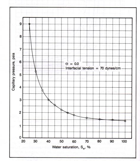
Solution to Example
3.4
First, convert the Pc lab to Pc res:
![]()
Next, convert Pc res to height above the free water table and plot on the right axis by putting
a new scale on the RHS for “h”. Its scale is 5.0 ´ the scale for Pc lab. This is shown below.
![]()
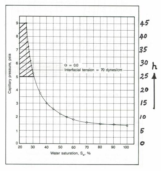
Mark off the top (45 ft) and bottom (25 ft) on the h-axis.
![]()
![]()
Since the area in this case can be approximated by a single trapezoid, the
shaded area
Therefore,
![]() = 0.28
= 0.28
The area under more complex shaded areas can be calculated after sub-division into a number of trapezoids and applying the trapezoidal rule.
3.5 Averaging Capillary Pressure Curves
Consider
a reservoir cross-section from which four core samples are taken at different
depth as shown below. Each core will generate its own complete capillary
pressure curve in the laboratory which can be converted to a reservoir
capillary pressure curve. Thus four different laboratory capillary pressure
curves are obtained as shown below. The question then arises:
How
do we get a single ![]() curve to represent the
reservoir?
curve to represent the
reservoir?
The
answer is to use the Leverett J-function
![]()
![]()
![]()
![]()

3.5.1 Leverett J-function
The
Leverett J-function is defined as:

where, ![]() = permeability
= permeability
![]() = interfacial tension
= interfacial tension
![]() = contact angle
= contact angle
![]() = porosity
= porosity
The
J-function has the effect of normalizing all curves to approach a single curve
and is based on the assumption that the porous medium can be modelled as a bundle of non-connecting capillaries (Slider
pp 279-280). Obviously the more capillary bundle assumption deviates from
reality, the less effective the J-function correlation becomes. This
correlation is not unique, but seems to work better when the rocks are classed
as to rock types, eg; limestone, dolomite, etc.
Given
several capillary pressure curves, with corresponding values of permeability ![]() and porosity
and porosity
![]() , the procedure for obtaining J-function curve is as follows:
, the procedure for obtaining J-function curve is as follows:
a) Pick several values of ![]() from 0 to 1 and read
the corresponding values of
from 0 to 1 and read
the corresponding values of![]() . There will be as many
. There will be as many
![]() values as there are
curves.
values as there are
curves.
b) For each ![]() value, calculate J and
plot versus
value, calculate J and
plot versus ![]() . Repeat for all
. Repeat for all ![]() values.
values.
c) Put your best correlation curve through
the data.
This
J-Curve is now a master curve that can be used to represent that reservoir and
in the absence of other data can be used for other reservoirs of similar rock
type. The graphs below, taken from (Amyx et.al.) shows the
J-function curve for the Edwards formation showing classification as to rock
types.
Fig. J-function correlation of capillary
pressure data in the Edwards formation, Jourdanton Field. J-curve for
(a) all cores; (b) limestone cores; (c) dolomite cores; (d) microgranular
limestone cores; (e) coarse-grained limestone cores. (Source
Amyx et.al.)
3.5.2 How to use the Leverett J-function to calculate Average Water Saturation
Values
for average initial or connate water saturation are required in many petroleum
engineering calculations. Examples are: (a) average water saturation in a section
of reservoir in order to fix effective fluid permeabilities, ![]() and (b) average water
saturation in the whole reservoir in order to fix the initial
hydrocarbon volume in place,
and (b) average water
saturation in the whole reservoir in order to fix the initial
hydrocarbon volume in place, ![]()
Under
capillary equilibrium conditions, the water saturation of a particular piece, or sample of rock not depends on several factors. It
has been shown with certain limitations, that a properly determined Leverett J-function
versus water saturation curve can be used to obtain an
average water saturation from a number of capillary pressure curves. It
is assumed that a Leverett J-function curve is available and applies to the
reservoir. The objective here is to show how to use the J-function to obtain
the best possible estimate of average saturation. Recall that the J-function is
defined as:

By
expressing the ![]() term in terms of
height and fluid densities the equivalent equation is:
term in terms of
height and fluid densities the equivalent equation is:

It
is important to note while applying this equation that its units are not
important. Mixed units can be used without appropriate conversion factors. It
is only important to be sure to use the same units that went into determining
the values of J making up the original plot. In other words, find out what
units were used to calculate the J-function curve and stay consistent with
those units whether they are mixed or not.
Note
also that J=constant*h. Therefore, the shape of a J-function versus ![]() curve would be similar
to that of a height versus
curve would be similar
to that of a height versus ![]() curve. The difference
is a displacement by a factor equal to the constant. Thus, a
curve. The difference
is a displacement by a factor equal to the constant. Thus, a ![]() curve can be converted
to a height curve simply by adding a new y-axis having its abscissa equal to
the constant*
curve can be converted
to a height curve simply by adding a new y-axis having its abscissa equal to
the constant*![]() .
.
3.5.2.1 Case 1: Permeability, Porosity, and Elevation are known for each sample

This
figure illustrates four reservoir samples having different values of
permeability and porosity and located at different heights above a ![]() datum. Assuming fluid
properties are the same in all pieces, the J-function equation can be
simplified to:
datum. Assuming fluid
properties are the same in all pieces, the J-function equation can be
simplified to:
![]()
3.5.2.2 The correct method
The
correct method of obtaining the average saturation, ![]() for the four pieces is
to calculate J for each piece, determine the corresponding water saturation,
for the four pieces is
to calculate J for each piece, determine the corresponding water saturation, ![]() of each piece by using
the J-curve and then taking the arithmetic average of the saturations with the
equation:
of each piece by using
the J-curve and then taking the arithmetic average of the saturations with the
equation:
![]()
Note
that this procedure correctly takes into account the vertical position of the
pieces and their corresponding permeability and porosity.
Less correct methods
These
methods first calculate average values of ![]() and
and ![]() , substitute them into the J equation to get an average J
value, and then read the average water saturation
, substitute them into the J equation to get an average J
value, and then read the average water saturation ![]() from the J-function
versus
from the J-function
versus ![]() graph. The only
advantage of these methods is that the amount of calculations is reduced. The
resulting
graph. The only
advantage of these methods is that the amount of calculations is reduced. The
resulting ![]() will always have error
in it. How much error depends on the specific condition being calculated. The figure below illustrates the concept behind
using average values in order to obtain an average J value.
will always have error
in it. How much error depends on the specific condition being calculated. The figure below illustrates the concept behind
using average values in order to obtain an average J value.
There
are two ways:
Method
(a): Calculate ![]() for each sample and
obtain the arithmetic average for all four. Also, obtain the arithmetic average
for each sample and
obtain the arithmetic average for all four. Also, obtain the arithmetic average ![]() . It is assumed that the average
. It is assumed that the average ![]() is located at the
average height
is located at the
average height ![]() . The average J-function equation then becomes:
. The average J-function equation then becomes:
![]()
where, ![]()

This
is the easiest of the averaging methods to do.
Method
(b):
The geometric average permeability and porosity are used to get the average
J-function:
![]()
![]() = geometric mean
permeability =
= geometric mean
permeability = ![]()
![]() = geometric mean
porosity =
= geometric mean
porosity = ![]()
Zero
values of ![]() and
and ![]() are not permitted when
evaluating the geometric averages. Because porosity values usually show very
limited range, the geometric average porosity,
are not permitted when
evaluating the geometric averages. Because porosity values usually show very
limited range, the geometric average porosity, ![]() , can be replaced by the easier to calculate arithmetic
average,
, can be replaced by the easier to calculate arithmetic
average, ![]() , with little loss of accuracy. Therefore, the form used by
most engineers is
, with little loss of accuracy. Therefore, the form used by
most engineers is
![]()
where, ![]() is the arithmetic average
is the arithmetic average
3.5.2.3 Errors due to using average values of  and
and 
Standing(4) discusses the
amount of error in ![]() introduced by using
average values of
introduced by using
average values of ![]() and
and ![]() and states that the
error depends on several factors.
and states that the
error depends on several factors.
One
factor is the distribution of ![]() in a vertical sense.
If the
in a vertical sense.
If the ![]() are distributed
randomly, no error will be involved. On the other hand, if high permeabilities
predominate in one portion of the section and low permeabilities in another,
some error will be introduced.
are distributed
randomly, no error will be involved. On the other hand, if high permeabilities
predominate in one portion of the section and low permeabilities in another,
some error will be introduced.
A
second factor is the shape of the ![]() curve. Where log J is
linear to
curve. Where log J is
linear to ![]() , no error will result from geometric average
, no error will result from geometric average ![]() . Where J is linear with
. Where J is linear with ![]() , some error will result.
, some error will result.
A
third factor is the range of permeability values. Little error is introduced
when the range is small and more error is introduced when the range is large.
The best way to minimize errors of averaging is not to average. Use the correct
method.
3.5.2.4 Case
2: Permeability and porosity are unknown as functions of elevation. Distance
from  (distance from
free-water table) is known
(distance from
free-water table) is known
The
petroleum engineer often needs to develop a value for average water saturation
but does not have detailed information on permeability and porosity as a
function of elevation. (Many wells are not core analyzed). However, he may know
from results of pressure buildup tests that the average permeability in the
region of the wellbore is, say, 100 md. Also, he may know from well logs that
an average porosity is, say 18%. With these average permeability and porosity
values plus information on the distance to the appropriate ![]() datum and information
on fluid properties, he can make a reasonable calculation of the average water
saturation.
datum and information
on fluid properties, he can make a reasonable calculation of the average water
saturation.
To
illustrate the method of getting ![]() , consider the sketch above. At the wellbore location, the
bottom and top of the formation are
, consider the sketch above. At the wellbore location, the
bottom and top of the formation are ![]() and
and ![]() from the
from the ![]() datum. For given
values of
datum. For given
values of ![]() , calculate
, calculate ![]() . Shade the area enclosed by
. Shade the area enclosed by ![]() and
and ![]() on the
on the ![]() curve and calculate
the average initial water saturation
curve and calculate
the average initial water saturation ![]() .
.
The
simplest way of determining ![]() is by graphical
integration. Thus, determine the area under the curve, divide this area by the
value
is by graphical
integration. Thus, determine the area under the curve, divide this area by the
value ![]() and the result will give
and the result will give ![]() . That is:
. That is:

Example 3.5
Example
calculation of the use of Capillary Pressure Data to Obtain Average Water
Saturation Using J-Function
It
is desired to calculate the initial oil in place for an oil reservoir having a
gas cap as illustrated below. There is no prior J-function curve available and
no well logs to give permeability, porosity, and saturation data with depth.
All we have are old cores from storage.
The
bulk volume of the oil zone is 1,000 acre-ft. The thickness of the oil zone is
20 ft. Four core samples were taken from the oil zone in the middle of 5 ft.
intervals. From laboratory measurements of porosity and permeability, the data
are:
|
Interval
depth |
Permeability |
Porosity |
|
4,000 -
4,005 |
11.2 |
0.147 |
|
4,005 -
4,010 |
34.0 |
0.174 |
|
4,010 -
4,015 |
157.0 |
0.208 |
|
4,015 -
4,020 |
569.0 |
0.275 |

The
free-water table is at a depth of 4030 ft. In addition to porosity and
permeability, the capillary pressure for each sample was measured using air
displacing water in a centrifuge. These laboratory
derived capillary pressure curves are shown below. The water/oil interfacial
tension for this reservoir is estimated to be 28 dynes/cm,
the reservoir (water/oil) wetting angle is 0.0. The air/water interfacial
tension is 70 dynes/cm with a wetting angle of 0.0 also, ![]() . Calculate the average water saturation and the initial oil
in place.
. Calculate the average water saturation and the initial oil
in place.
Solution
a) Convert the ![]() data to
data to ![]() data and calculate the J-function curve using:
data and calculate the J-function curve using:

This
has been calculated and plotted below.
b)
Calculate the value of ![]() at each "
at each "![]() " of each core and read the corresponding water
saturation from the
" of each core and read the corresponding water
saturation from the ![]() curve.
curve.
![]()
|
|
|
|
|
27.5 |
0.738 |
0.37 |
|
22.5 |
0.967 |
0.35 |
|
17.5 |
1.478 |
0.29 |
|
12.5 |
1.748 |
0.27 |
c)
Obtain the arithmetic average water saturation.
The
average water saturation ![]()
Using
the Less correct method
![]()
![]()
![]()
![]()
Therefore,
![]() by reading on the
J-function curve at
by reading on the
J-function curve at ![]()
Only
![]() and
and ![]() available
available
Suppose
there are no cores, there are no well logs, an average ![]() is available from well
tests, and
is available from well
tests, and ![]() can be estimated from
correlations.
can be estimated from
correlations.
In
this case, use the heights of the top and bottom of the pay zone from the
free-water table to obtain ![]() and
and ![]() .
.
![]()
Similarly, ![]()
Plot
these and find the average water saturation graphically.
Exercises
1.
Give a possible reason why ![]() for a
soap solution is about 40 dynes/cm and not about 70 dynes/cm as would be
the case for fresh water.
for a
soap solution is about 40 dynes/cm and not about 70 dynes/cm as would be
the case for fresh water.
2.
Show that the expression ![]() derived for a tube is
a special form of the general expression:
derived for a tube is
a special form of the general expression: 
3.
Given that ![]() and
and ![]() , would you expect a water/air interface or an oil/water
interface to have a smaller contact angle assuming the same capillary pressure
applies to both, in the same capillary tube.
, would you expect a water/air interface or an oil/water
interface to have a smaller contact angle assuming the same capillary pressure
applies to both, in the same capillary tube.
4.
Calculate the entry pressure for natural gas into a pore throat having the
following sizes and shapes.
a)
A cylindrical shape pore throat of 0.0001 inch diameter
b) An elliptical
shape pore throat of d1 = 0.0001 inches and d2 = 0.001
inches

c)
An infinite horizontal fracture of fracture width = 0.0001 inches.
Use
s = 35.2
dynes/cm, and q = 0.0
References
1.
Clark, Norman J. "Elements of Petroleum Reservoirs"
Henry L. Doherty Series, Society of Petroleum Engineers of AIME, Dallas, 1960.
2.
Slider H.C., “Worldwide Practical Petroleum Reservoir Engineering Methods”,
Penwell Books, 1983
3.
Wilhite, G.P. : “Waterflooding”, SPE Textbook Series,
Vol. 3, 1986.
4.
Standing, M.B.: Lecture notes,
5.
Amyx, J. W., Bass, Jnr. D. M., Whiting, R. L. :
Petroleum Reservoir Engineering, McGraw-Hill, 1960