 where:
Purpose
The purpose of this lab is to become familiar with the various operating characteristics of a G-M counting setup by completing the following objectives:
Obtain the Geiger Counting Plateau
Obtain the system dead time
Obtain the overall detection efficiency
Equipment
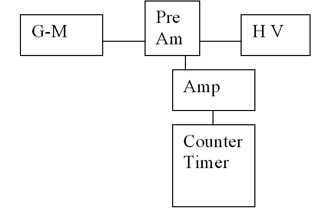
Basic Setup Lab Experiment Setup Diagram
Place the detector in some convenient location where it will not be moved throughout the experiment.
Obtain a Cs-137 source from the TA, and place it near the middle of the detector.
Once your first measurement of counts has been taken, do not change source-to-detector geometry; if the source is moved while data is being taken, your results will be skewed.
Experimental Procedure
A. Geiger Counting Plateau
1. Starting Voltage
Determine the starting voltage by first setting the scalar to count for a long period of time (flipping the switch from “0.01 sec” to “0.01 min” should accomplish this). Begin increasing the HVPS setting. At the first sign of an indicated count on the scalar, stop increasing the voltage. This voltage is the ‘starting voltage’ of the detector.
2. Continuous Discharge Voltage
Again, set the scalar to count for a long period of time. Increase the HV by approximately 200V, and note the rate at which the counts on the scalar is increasing. If the scalar is increasing too quickly, you may increase the distance between the source and the detector to lower the count rate. Slowly increase the HV setting. As soon as you notice the scalar showing a rapid increase in the counting rate, note the HV setting, and reduce the voltage. When the scalar shows a rapid increase (beyond what is expected by the source), the detector has entered its ‘continuous discharge region.
Counts vs. High Voltage
Reduce the HV to the nearest 20-volt setting that is just below your starting voltage. Set the scalar to count for 3 minutes (180 seconds).
Begin taking 3-minute counts at every 20-volt increment until you reach the continuous discharge region. When taking counts near the starting voltage, if you do not receive any indicated counts within the first minute, you may assume the counts are zero for that point and increase the voltage by 20.
Plot the counts vs. voltage to obtain a curve.
B. Dead Time
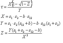
The dead time, t, will be computed using the two source method. This is valid if we assume the dead time is given by the Nonparalyzable model. It is computed from the following equation (it is also provided on page 122):
where:
Return your HV to a setting that is at the lower end of the voltage plateau (usually about 100 volts above your starting voltage). With your source reasonably far away from the detector, take a 5 minute background count. This count will be B, and its associated count rate will be b.
Place a Cs-137 near the middle of the detector and take a 5 minute source count. This count will be S1, and its associated counting rate will be s1.
Without moving the first Cs source, place another Cs-137 source near the middle of the detector. Take another 5 minute count. This count will be S12, and its associated counting rate will be s12.
Finally, remove the first source (without moving the second), and take another 5 minute count. This count will be S2, and its associated counting rate will be s2.
System Efficiency
The efficiency of the counting system is given by the following equation:

A0 is the initial activity, t is the decay time, and t^1/2 is the half-life of the source. You will be given this information. s is the net counting rate obtained from your dead time measurements. Compute the efficiency of the system for both s1 and for s2.
In addition to providing the data requested above, the following questions should be addressed in your lab report:
What is the significance of the Geiger Counting Plateau? Why does this phenomenon make a G-M detector ideal for use as a ‘simple counter?’
What accounts for the sudden increase in the count rate between the starting voltage and the ‘knee’ of the voltage plateau?
Why is it important to know the continuous discharge voltage? What effect would operating in this region have on your count rates? What effect would operating in this region have on the detector?
In the dead time section, you were instructed to place your voltage setting at the lower end of the voltage plateau. What is the advantage of operating the detector at this region, rather than at some higher voltage if the count rate will be the same?
Following equation: ![]() gives an approximation to the dead time equation (with the assumption that the background rate is zero). How does this dead time approximation compare to the actual dead time you determined previously? What is the relative error between the two measurements?
gives an approximation to the dead time equation (with the assumption that the background rate is zero). How does this dead time approximation compare to the actual dead time you determined previously? What is the relative error between the two measurements?
Best results for dead time determination are obtained if the sources are active enough to obtain a fractional dead time, s12t, of at least 20%. What is your value for the fractional dead time?
What factors are relevant for the system efficiency (i.e. what factors would change the efficiency of a radiation measurement)?
What would account for the difference in system efficiency between the two