|
Highlight the second column of your data. This will be the
dependant (Y) varible of your graph.
|
 |
|
| Now click the chart wizard button. | 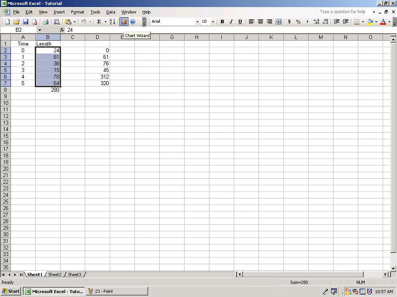 |
|
| The chart wizard will open. | 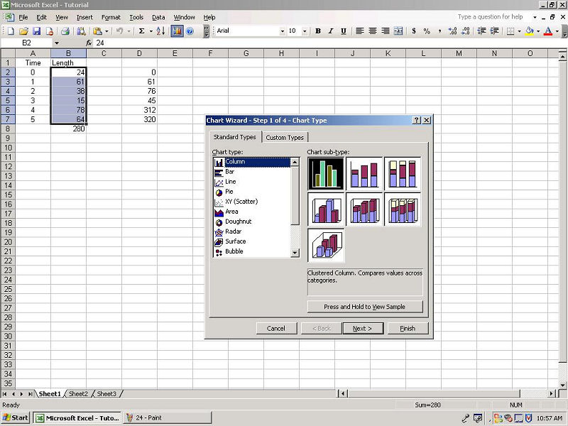 |
|
| There are many different graphs available in Excel. Today, we will use the line graph. Select the line option from the column on the left. From the box on the right select an appropriate chart subtype. We will choose a line type that features markers. | 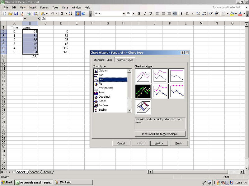 |
|
| To see a preview of your graph press and hold the preview button. | 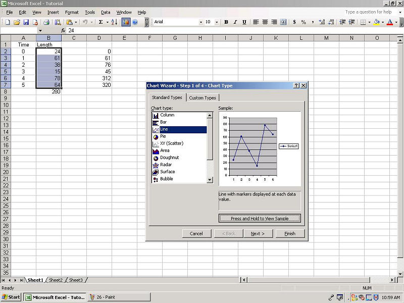 |
|
| Now click Next. A screen will appear allowing you to customize your graph's data range and if you want this data in rows or columns. Since we selected our data before starting, we do not need to change any of these options. | 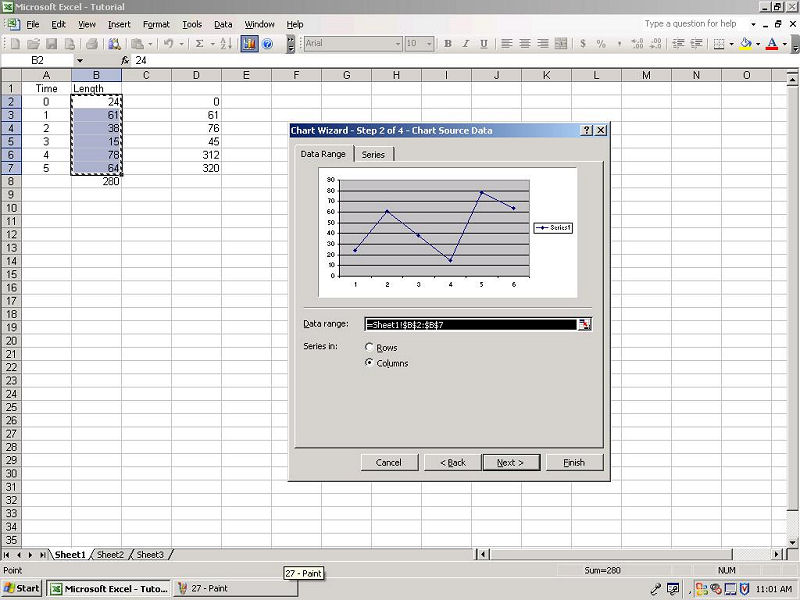 |
|
|
Now click on the Series tab, which can be found at the top of the dialog
box.
|
 |
|
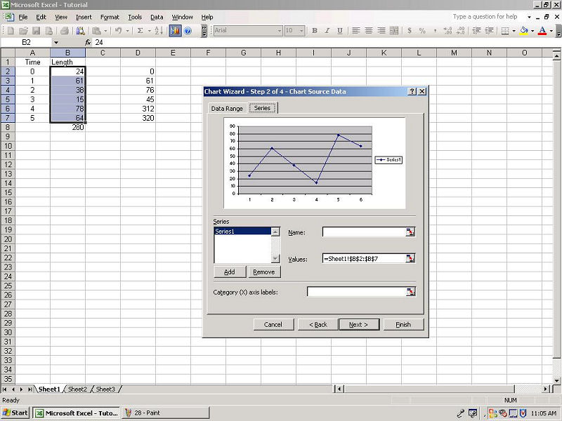
| This section allows you to name your dependant (Y) variables and select which values you want to use for your independent (X) variables. We will type "Length" in for name. Click the button to the right of the Category (X) Axis Labels. | 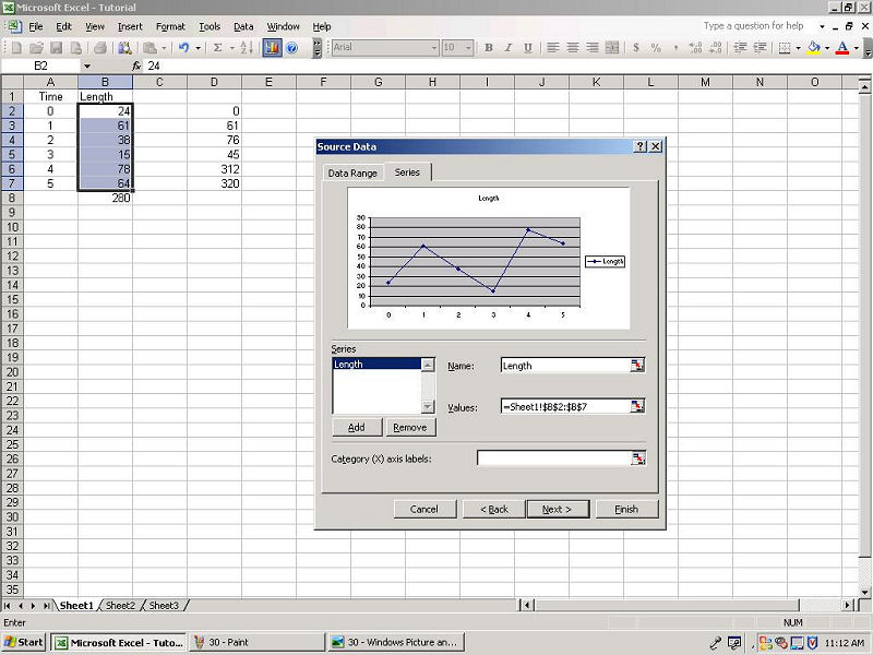 |
|
|
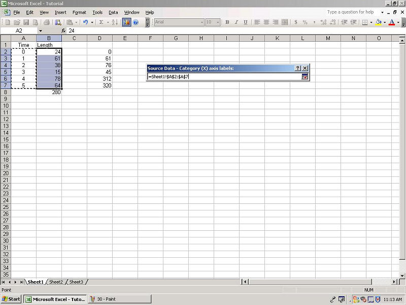
Select the values that you want to use for your dependant (X) variables
from the main portion of the spreadsheet.
|
 |
|
| Now click on the button to the far right of the new window that opened to select these values and return to the Series tab. Your new values will show on the graph preview and you will now have data in your Category (X) axis labels box. | 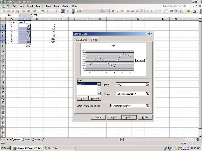 |
|
| Now click Next to bring up the Chart Options window. | 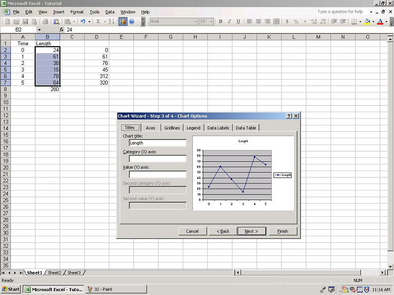 |
|
|
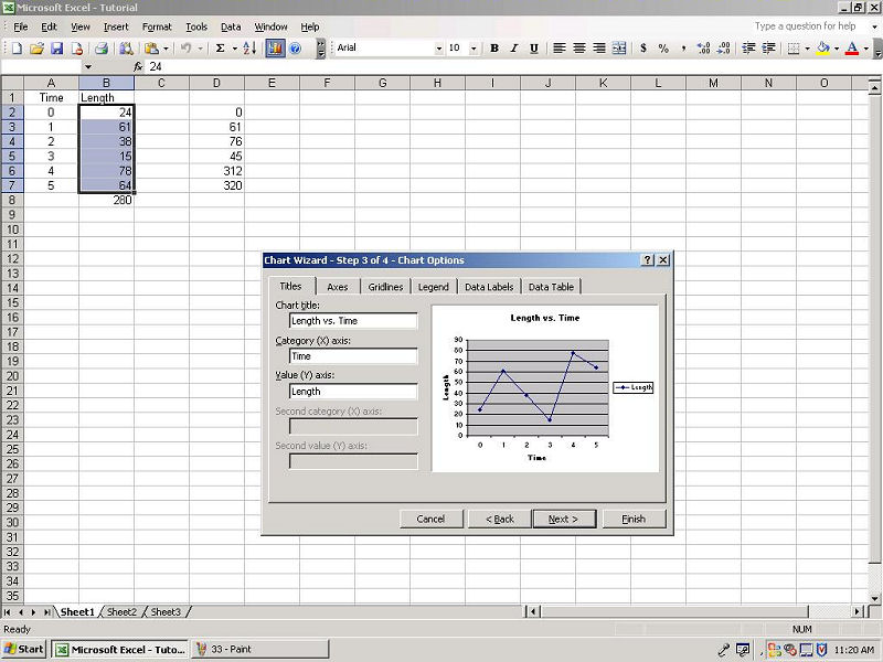
This box allows more customization of your chart. The first tab is
Titles. We will type in "Length vs Time" in the Chart
title box. Next we will type in "Time" for the Category
(X) axis box and "Length" for the Value (Y) axis box.
|
 |
|
| Now click Next. This will bring up the final window for our chart. It allows us to select whether we wish to place our new chart into the spreadsheet with our values, or as its own page. | 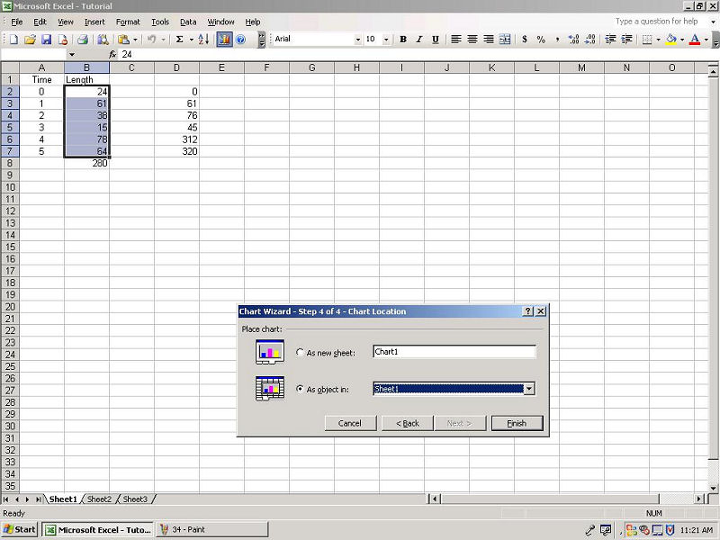 |
|
| We will place it in our original spreadsheet by choosing the bottom option and selecting Finish. | 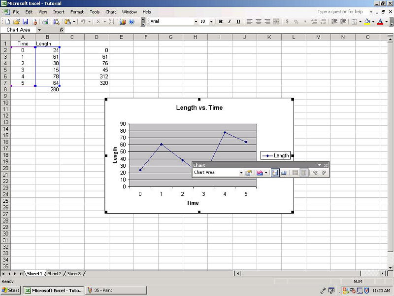 |
|
|
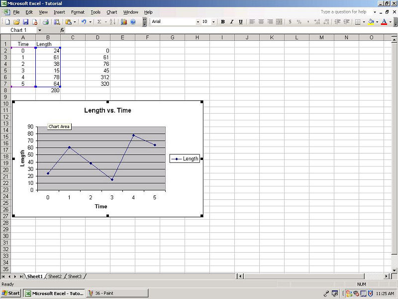
Your chart will appear in your spreadsheet, along with a new window.
Exit out of this window. This window can be moved or resized at
will. To move it, click and hold your left mouse button and drag it
to your desired position. Then, release your mouse button.
You may also edit your graph's options by double clicking on almost any portion of the graph. This includes the titles, the X and Y values, and even the graph legend and the line itself. These options are numerous and can provide many hours of serious entertainment for even the casual Excel user. Congratulations, you have finished your graph!
|
 |