Linear Regression
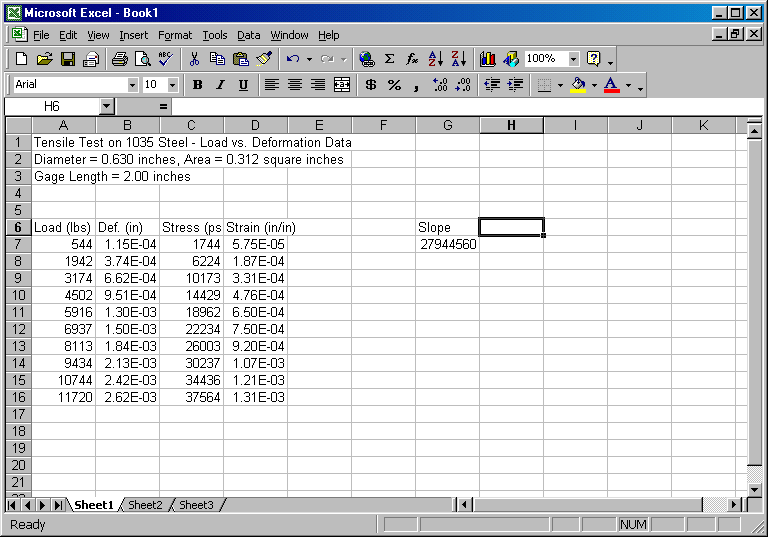
Now that we have generated our stress vs. strain data, we would like to generate a best fit line of the data (i.e. a linear regression curve). Move the curser to cell G6 and type Slope. Repeat this for cell H6 with Y-Intercept. Now type +INDEX(LINEST(C7:C16,D7:D16),1) in cell G7 and press enter. This formula will return the slope for the stress (C7 to C16) and strain (D7 to D16) data. Note the arrangement of these cell designations in the formula. The formula has the following form: +INDEX(LINEST(known y's,known x's),1), where stress is considered the known y values and strain is considered the known x values. This will make more sense when we plot stress versus strain in a moment. Currently, your spreadsheet should look like the following:

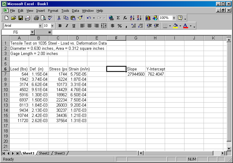
Repeat this procedure to determine the y-intercept using +INDEX(LINEST(C7:C16,D7:D16),2). The only difference between this formula and the slope formula is the last digit. If this digit is 1, Excel will return the slope, and if this digit is 2, the y-intercept will be returned. Your spreadsheet should look like the following:

If we want the linear regression line to appear on the graph, we will now have to generate the linear stress data corresponding to the experimental strain values, i.e. the theoretical y values for the given x values. That is, we need to generate the values of
stress = m (strain) + b
( i.e. y = m x + b ) where the m is the slope b is the y-intercept.
Label cell E6 as LinRegStr (for linear regression stress). Now move the cursor to cell E7, type +$G$7*D7+$H$7, and press enter. This equation multiplies the slope stored in G7 by the strain value in D7 and adds the y-intercept stored in H7. The $ signs anchor the slope and y-intercept cells so that they will not increment when we copy the equation to other cells.
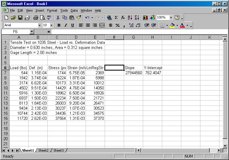
Now select E7, click on Copy. Highlight E8..E16 and click on Paste. You should now see numerical values of stress in column E. These values will be used in conjunction with the strain values to plot the linear regression line. Before proceeding, clean up the formatting by highlighting E7..E16, click on Format, Cells..., Number, Number, and select 0 decimal places and OK. Your spreadsheet should now look like the following:

Our computational work is now complete. All that remains is to display the data in the graphical format of our choice.