The curve fitting method of least squares involves minimizing the sum of the squares (S) of the vertical deviations (v) of the plotted points from the fitted curve (Fig. 1).
where
and n = number of data points.
Straight Lines by Method of Least Squares
Many physical problems involve fitting a curve to a set of experimental data points. The simplest, and probably the most important curve used to fit data is the straight line. Unfortunately, many people can not "eyeball" a decent straight line through even an excellent set of data points. Inability to visualize a good curve fit need not hamper the industrious student, since a mathematical curve fitting technique may be employed. One thus replaces individual subjective judgment with an objective mathematical technique.
The primary problem in selecting a curve fitting technique is to determine the criterion which will give the 'best possible fit'. By far, the most widely used mathematical curve fitting technique is the 'method of least squares'. This method is generally used when the statistical distribution of error is unknown, or where it is thought to have a 'normal' distribution. In the case of a normal distribution of error, the method gives statistically the 'best possible fit'. It is important to note that errors in measurement generally have a normal distribution.
The method of least squares requires that the sum of the squares of the vertical deviations of the experimental data from the fitted curve be a minimum. Analysis of the resulting equations shows that the method also requires that the sum of the vertical deviations be zero. The method can be used to fit curves other than straight lines, but our attention will be confined to the straight line.
The curve fitting method of least squares involves minimizing the sum of the squares (S) of the vertical deviations (v) of the plotted points from the fitted curve (Fig. 1).

where

and n = number of data points.
For a straight line,

For minimum S,


and

Therefore

and

Rearranging the order of summation we obtain a more convenient form of the equations:


The last two equations must be solved simultaneously for m and b. The solution results in the least-squares best fit line: y = mx + b.
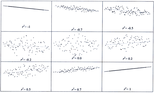
While calculating the least squares parameters we generally also determine a parameter which gives a measure of goodness of fit. The correlation coefficient (r) is such a measure. It compares the goodness of fit of your straight line to a horizontal line which passes through the mean (ymean) of the data set. The correlation coefficient compares the sum of the squares of the vertical deviations with the sum of the squares of the deviations of the data points from the mean value,

If the curve exactly fits the data points then
is zero and the correlation coefficient r = ± 1 indicating a perfect fit. If the fitted curve gives no better fit than an arbitrary horizontal line through the mean then r will be near zero, with zero telling us there is in effect no reason to expect a linear function to represent the data!
Interpretation of r for intermediate values (i.e. not near 1 or 0) is more difficult. There is however a simple way to gain some insight as to the significance of r. If the value of r is squared and multiplied by 100 it represents the percent of the variation of the y values that can be attributed to the variation in the x values. For example if r = 0.8 then 64 percent (100% x r2) of the variation in the y values can be attributed to the variations in the x values. The remaining 36% of the variations in y is due to such things as experimental errors, nonlinearity of the physical relationship between the variables or partial dependence on other varying parameters.

from Product Design - Techniques in Reverse Engineering and New Product Development, by K. Otto and K. Wood, Prentice Hall, 2001, page 939.
To facilitate computation, r is usually calculated from the following equation. It can be shown to be equivalent to the previous expression, but this form is more convenient.
