STEP Solar Thermal Electric Panel
Results
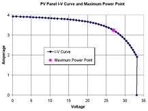
Figure 6: The I-V Curve
The PV power output was obtained by finding the maximum power point on the I-V curve. This technique was used because find a consistent load and the cost of inverting equipment would have been more expensive.
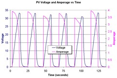
Figure 7: A Sample Set of PV Data
Forty-eight data points are taken at each capacitor bank charging cycle to obtain the maximum power the PV is outputting. Figure 6 shows the I-V curve over a ten second charging interval. Figure 7 shows the voltage and amperage plotted versus time.
Since only one panel is tested at any given sample interval the output would only be one sixth of what the whole array would be seeing. To validate the multiplying each sample by six to simulate whole array production the six panels were plotted with each other to see how well match they were. Since the average standard deviation between all of the panels were only about 2 Watts, which is a low percentage compared with the total, it was deemed valid to make the assumption and institute this scaling factor. Figure 8 shows the PV panel comparison that validates the use of the scaling factor.

Figure 8: PV Panel Comparison
Over the four hour testing period, for two hours before solar noon and for two hours past solar noon, the PV array collected about 2.4 kilowatt-hours (kWh). Figure 9 shows the energy gain during its sampling interval compared to the available radiation striking the collector surface. There should be, and is, a direct correlation to energy gain and available radiation.

Figure 9:Energy Gain Interval
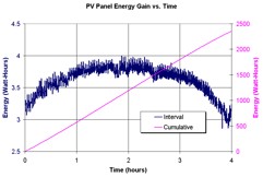
Figure 10: Interval and Accumulation
Please note that solar noon is at the two hour mark. Figure 10 shows the same energy gain interval curve with a comparison to the cumulative energy gain throughout the four hour sampling period. As stated before, at hour four the accumulation is 2.4 kWh.
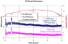
Figure 11: Glazed PV Behavior
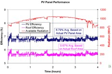
Figure 12: Unglazed PV Behavior
The efficiency of the solar panels in the STEP system averaged around five percent. Figure 11, on the next page, is a good representation of PV panel performance on an average sunny day; the daily temperature of all seven test days average to 70°F. The plot also shows the difference in areas. The two areas being the area only the solar panels encompass and the area of the whole collector as it sits on the roof. At about a half hour into this test, an increase of efficiency is noticed while the available radiation is decreased. This could be due to the affect of heat on the solar panels. The same trend is seen on the test day where the glass was removed from the collectors. Figure 12, on the next page, is the plot of the PV performance data with the glass removed from the collector. There are multiple occasions during this test where the efficiency increases with a decrease in radiation. This behavior seems to be counter-intuitive. Also, the efficiency of the photovoltaic panels decrease due to the glazing of the STEP system. The panels decreased in efficiency by 23% going from 6.79% to 5.22% which is a difference of 1.57%.
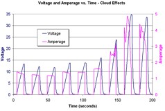
Figure 13: Cloud Effects in the PV's
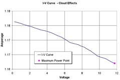
Figure 14: Cloud Effects on I-V Curve
Since the collector will not see cloudless days every day, a test day of cloudy weather was sought after. The validation of the capacitive I-V tracer could not be established. Instead of the nice arc of the previous I-V curve, shown in Figure 6, the relationship between the voltage and the amperage is almost linear. This linearity is due to the construction of the solar panel itself. The PV panel has shading protection built in. Meaning if one portion of the panel was shaded the whole panel would not be affected just the area the was under shade; sort of like the old Christmas lights in a string, if one was bad the whole string would not light. This protection is done by diode bridging. So on a cloudy day the panels act as if they were being shaded and the amperage is held to a constant for amperages below about 2 amps where the maximum amperage for the solar 5 amps. Figure 13 demonstrates the squaring off of the amperage during cloudy conditions. Figure 14 is the I-V curve created panel is from the squared off amperage data from Figure 13. The point never reaches a maximum so for this test the cloudy I-V curve is invalid.
Now that the electric side of the STEP hybrid system has been explored, the results thermal side of the system will be presented in a similar fashion. First off, all of the thermal panels are assumed to be identical since all six of the panels are joined by an upper and lower header. This means the thermal system has one input and one output. The temperature is measured just before the fluid enters the collector area and after the fluid leaves the collector area. Unlike a normally operating system, this test ran the pump throughout the experiment. Usually you would only run the pump when the fluid in the collector is at a higher temperature than the fluid in the tank; this would be accomplished by using a differential controller with a setback. The reasoning behind running the pump the whole time is to explore what happens during that transition between inlet and outlet temperatures. As a reminder, Figure 3 shows the hot water circulation schematic.
Unlike find the energy collected through PV panels, the energy collected through the thermal panel requires other elements such as the thermal capacity of the fluid, the fluid flow rate and the density of the fluid. Equation (1) shows the general form for the energy gain for the thermal system.
(1)
Since the fluid is half anti-freeze and half distilled water the specific heat and density was formulated by taking the average of both fluids; the density is needed for a conversion factor. The Dow Frost had a range of values for different temperatures so the average of the test temperature range was used. Equation (2) is the final formula used for thermal energy gain. This formula contains all of the conversion factors and the specific heat so the fluid flow rate and the temperature difference can be plugged in from the data received from the data logger.
(2)
Efficiency of a thermal collector is not an easy number to produce. Unlike with PV production, many more factors affect its performance. An easy way to think about this is if your inlet temperature is lower than the outside, ambient temperature, the collector will show more efficiency when comparing energy gain with available radiation. Conversely, if the inlet temperature is greater than the ambient temperature then the efficiency with drop dramatically. But, this is good energy production because we need to get the water to above 120°F to be useful for household needs.

Figure 15: Thermal Energy Gain
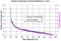
Figure 16: Change in Temp. and Efficiency
This experiment used a hot water tank where thirty gallons where cycled through the collector at about four gallons per minute; thirty gallons of water is about enough for one and a half people on a typical usage day. Figure 15 shows the typical production over the test interval and the accumulation. The peak of production being just over 2.5 kWh. Remember that the PV panels produced 2.4 kWh over their four hours of production. The total production can be increased by using the aforementioned differential controller with setback. As mentioned previously the efficiency of a thermal panel is primarily dependant on where the inlet temperature is compared with the ambient temperature. Figure 16 plots the thermal efficiency with the change in temperature compared to the inlet temperature. Note that these curves are identical. So the change in temperature between the inlet and the outlet is directly proportional to its thermal efficiency at any given inlet temperature. As a reminder, the average ambient temperature was 70°F.
Similarly to the PV plots, Figure 17 shows how the inlet and outlet temperatures compare with the available radiation. As the fluid heats up the temperature difference diminishes due to the extra energy needed to overcome the ambient conditions.

Figure 17: Inlet and Outlet Temps.
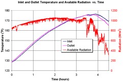
Figure 18: High Starting Inlet Temp.
Unlike the PV system the thermal system does not track with the available radiation. Heat is built up and
after the greatest heat of the day and reaching its maximum potential the inlet temperature will drop below the outlet temperature. The maximum temperature achieved from circulating the thirty gallons of water approached 160°F. The peak occurred at about one hour past solar noon. These results would be skewed if the starting inlet temperature was higher or lower. Figure 18 shows this result of a high starting inlet temperature. The output surprisingly had approximately the same amount of gain. The peak did occur well after the three hour mark. If the radiation was not obscured by clouds the maximum temperature, of 177°F, and the inlet and outlet convergence could have possibly been extended. With that in mind, every day is never identical to the previous one. The thermal energy production for this day peaked at 1.7 kWh compared to the lower starting inlet temperatures peak of 2.5 kWh. This is due to the lower thermal efficiency at higher temperatures.
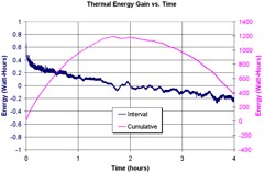
Figure 19: Unglazed Energy Gain
As done with the PV side of the system, the thermal side will compare the glazed system to the unglazed system. Using Figure 15 as the glazed comparison, Figure 19 shows the effects of energy gain with glass covering the collector. The glazed collector has the means of trapping the suns radiation which not only amplifies the heat via the greenhouse effect but also extends the heat collect period. Figure 19 shows that its performance depends on the available radiation. The pink bell shaped curve mimics the available radiation with solar noon occurring at time equal to two hours. In figure 17 where the inlet and outlet temperature converge is about the peak of production for the test period. Similarly the convergence for the unglazed system occurs at solar noon. Note that the maximum energy production of the unglazed collector only reaches 1.2 kWh where the glazed collector, with comparable ambient and inlet temperatures, achieved 2.5 kWh.

Figure 20: Cloudy Thermal Performance
Most thermal collection systems do not work very well in cloudy weather. Even an evacuated tube collector has a big disadvantage. The biggest problem is most of the suns radiation does not make it to the collector surface. The ambient temperature plays a large role in how much energy can be obtained in cloudy conditions. The ambient temperature for this test day averaged 80°F. Figure 20 shows the results of the data collected on this cloudy day. The squiggly red line denotes the clouds moving across the collector surface; in bright sun a value of 1050 Watts per square meter was measured. Even though this day was significantly cloudy the thirty gallons of fluid was heated to above the domestic hot water mark of 120°F. If this measurement was taken on a much colder day the fluid would not be able to reach the domestic temperature due to the ambient air drawing the heat away from the collector. Also, if the thermal system was unglazed the result would be much poorer because the suns radiation that did peak through a cloud would not be stored behind the glass.

Figure 21: With Stagnation

Figure 22: Without Stagnation
Before looking at the comprehensive test data plots, one more test that was carried out will be addressed. It is well known that solar panels perform better when they are cooler. Since amorphous panel technologies are relatively new, not much data has been acquired about their thermal performance. Some previous experiments by this researcher and the manufacturer has shown that a temperature, in the range covered in this report, does not have as much of an effect on amorphous panels as it does on mono- or poly-crystalline panels. To achieve this in our experimental setup the fluid pump was not run. The glazing is on the collector so the greenhouse effect is still in play. With no fluid flow the PV panels would see a higher temperature. Figure 21 shows the performance of the PV panels with the effects of stagnation while Figure 22 does not take stagnation into account. While there is some difference in the efficiencies, it could not be stated as fact that stagnation, or higher PV temperatures, effected this output due to varying conditions.

Figure 23: PV Efficiency Curve
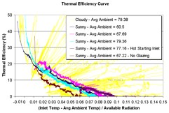
Figure 24: Thermal Efficiency Curve
Now to combine all of the data into two plots to help characterize the STEP system. First the electric plot, shown in Figure 23, shows the performance curve. With all of the efficiency data plotted with its corresponding radiation number, a curve can be made out. This curve could be used to estimate efficiency therefore energy collection for differing available radiation conditions. Note that the teal colored data does not fit this curve. This data is taken from the test day that had no glazing on the collector so it would be its own curve. Figure 24 shows the thermal results from all of the testing days. Using this curve data different seasonal scenarios can be observed.